Cosmological model with variable speed of light **
COSMOLOGICAL MODEL WITH VARIABLE SPEED OF LIGHT:
INTERPRETATION OF REDSHIFTS.
**
Jean-Pierre PETIT.
Marseille Observatory
Physics Letters A, Vol.3, No. 18, Dec. 1988, p.1733
ABSTRACT:
The model with variable c, G, h presented in reference [1] is extended to electromagnetism. The entropy is found to be proportional to Log t and, in a space-entropy representation, the metric is conformally flat. A new gauge relation is proposed, based on geometrical considerations, corresponding to a Rydberg constant varying as R. Hubble's law still applies. The age of the universe remains unchanged while its span is found to be half of the Mattig value. The complete decoding of the redshift becomes possible. The distances of the sources are very similar. The volumetric power densities of distant quasars could have been greatly overestimated, while the increase in their absolute magnitude, as derived from classical theory, could be due to the secular variation of c. Assuming that the electron-proton mass ratio varies as R, we obtain a fine-structure constant α, a Bohr radius, and a ratio of electromagnetic force to gravitational force that behave as absolute constants.
1 - INTRODUCTION
...Several authors have attempted to develop models with physical constants varying in time [2, 3, 4, 5, 6, 7, 8, 9]. None questioned the speed of light c, always considered an absolute constant. If one wishes to preserve the form of the conservation equations, the Einstein constant κ = - 8πG / c² must be considered an absolute constant. Under these conditions, if one wishes to keep the speed of light c as an absolute constant and have a variable gravitational constant G, one must add a source term to the field equation, see reference [3]. Thus, all these theories imply a constant creation of matter.
...In a previous paper [1], we showed that a variable speed of light could lead to a consistent model if G and the Planck constant h followed suitable gauge relations. Thus, the constant creation of matter was no longer necessary. The extension of the Robertson-Walker metric to a variable speed of light configuration, and its introduction into the field equation, yielded a complete set of gauge relations. Let us recall the main features of the model described in [1]:
(1)
(2) m (particle mass) ∝ R
(3) h (Planck constant) ∝ R³/² ∝ t
(4) G (gravitational constant) ∝ 1/R
(5) R (characteristic length) ∝ t²/³
(6) V (velocity of a free particle) ∝ R⁻¹/² ∝ c
(7) ρ (mass density) ∝ 1/R²
(8) mc² = constant
The following is a brief digression on entropy.
- TIME OR ENTROPY?
The relativistic formulation of the velocity distribution function is:
(9)
where m is the rest mass, T the temperature, n the number density, and K₂ a Bessel function. If β = (<v²>¹/²/c) << 1, we obtain the classical Maxwell-Boltzmann distribution function: (10)
Let us compute the entropy per baryon, defined by: (11)
where k is the Boltzmann constant. We have n ∝ R⁻³, m ∝ R, and R ∝ t²/³, T = constant (see reference [1]), such that: (12)
Then: (13) s = k Log t + H(β)
In the model, β is gauge invariant, so s ∝ Log t.
...In classical cosmology, the universe is isentropic. One might find it somewhat paradoxical that such an enormous change in time is accompanied by an almost zero variation in entropy. In the new model, entropy grows with time. Note that the BIG BANG singularity corresponds to s = - ∞.
Let us now define the entropy by: (14) s = 3/2 k Log t
Returning to the Robertson-Walker metric (15)
We obtain: (16)
...In the {entropy, space variables} representation, the metric is conformally flat. From a cosmological point of view, entropy (which, moreover, is invariant under Lorentz transformations) could be a better choice than time. ...Furthermore, if we describe the universe in phase space (position plus velocity), we find that the characteristic hypervolume R³c³ varies as t.
- THE REDSHIFT AND THE ROBERTSON-WALKER METRIC:
...Consider a radiating object, say a nebula N₁, which can be considered as a particle. Suppose its light is observed on a nebula N₂ placed at the origin of the comoving coordinates. The nebula N₁ is characterized by the value of its time-independent distance marker z, defined by the relation:
(17)
The light emitted at time t₁ is observed on N₂ at a time t₂ with t₂ > t₁.
The distance between N₁ and N₂ is R(t) dz and is time-dependent, but dz is not. Light propagates along a null geodesic: (18)
ds² = (dx⁰)² - R² dz² = 0
Consider the light emitted by N₁ at a corresponding value x⁰₁ + Δx⁰₁ of the chronological parameter. It will be received at x⁰₂ + Δx⁰₂, where it will be determined by the relation: (19)
...Consider Δx⁰₁ as the equivalent of the period of some physical phenomenon, such as the emission of radiation, taking place on N₁, and Δx⁰ to be short compared to the equivalent of the travel time from N₁ to N₂ (in terms of the chronological parameter x⁰). The periodic phenomenon will appear, as seen from N₂, to have a "period" Δx⁰₂ such that, from the above relation, the increment of the integral q will be zero. This, by elementary calculus, gives: (20)
Introduce the cosmic time t defined previously by dx⁰ = c dt and denote R(x⁰₁) = R₁, R(x⁰₂) = R₂, c(x⁰₂) = c₂, c(x⁰₁) = c₁, we obtain:
(21)

- THE PROBLEM OF ELECTROMAGNETISM:
...We can no longer assert that the energy Eᵢ(t₁), emitted by the atom at time t₁, would be identical to the corresponding emission energy Eᵢ(t₂) of a similar atom, at time t₂, under laboratory conditions. Light emission is an electromagnetic phenomenon. Everyone knows that the classical field description, applying to a four-dimensional spacetime, does not account for the electromagnetic phenomenon. To obtain a complete description of the universe, gravitation and electromagnetism should be embedded in a common geometrical framework. Unfortunately, this has not yet been done satisfactorily, so our work loses some of its internal consistency. Suppose, for example, that the Rydberg constant (ionization energy of hydrogen) simply obeys the following hypothetical gauge relation: (22)
Eᵢ ∝ Rᵍ
(Note that this is a totally arbitrary assumption). Let us explore the consequences of this assumption on the decoding of the redshift. Later, we will try to relate it to possible gauge relations.
- THE REDSHIFT PHENOMENON:
...In the classical description, the redshift z is due to the Doppler effect, plus an additional special relativity effect. The subscript 1 refers to the emitter and the subscript 2 to the receiver. For a given spectroscopic line, let E₁ = h₁ν₁₀ be the emission energy and E₂ = h₂ν₂₀ the corresponding emission energy under current laboratory conditions for the same line. The light is emitted by an atom at rest at the frequency ν₁ = ν₁₀, corresponding to the wavelength λ₁ = c₁/ν₁ = λ₁₀.
ν₂ will be the measured reception frequency, with λ₂ = c₂/ν₂ and λ₂₀ = c₂/ν₂₀. The energy of any radiative process will follow the general assumed gauge law (22).
We can define the redshift z:
- As the ratio between the wavelengths:
(23)
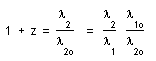
(24)
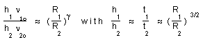
(a)
(b)
(c)
we obtain:
(25)

Note that, for g = 1, we recover the classical model.
- As the ratio between the frequencies:
(26)
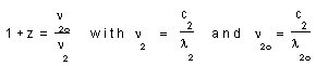
we obtain the same result.
- As the ratio between the energies.
(27)
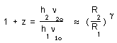
the same thing. The classical relation suggests the choice g = 1.
- HUBBLE'S LAW AND THE ROBERTSON-WALKER METRIC:
Expand the function 1/R(t) into a series with respect to
(28)

we obtain:
(29)
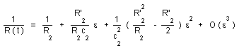
In R'² and R"², the prime denotes differentiation with respect to t. In particular, at first order:
(30)
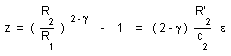
Next, expand the following expressions:
(31a)
(b)
(c)
Referring to the first order:
(32)
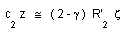
As a first approximation, the astronomer measures d₂ ≈ R₂ z, such that:
(33)
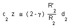

Which is nothing but Hubble's redshift law, which still applies in this variable speed of light framework. From the measurement of d₂, c₂, and z, we can derive the Hubble constant, i.e., the age of the universe.
Take R = 3/2 c t (see reference [1]).
(34)

The age of the universe corresponds to:
(35)
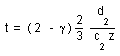
A value g = 1 gives the standard model value.
- THE REDSHIFT AND THE EVALUATION OF DISTANCES:
Return to the Robertson-Walker metric, which provides:
(36)
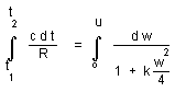
In the classical approach, take the Einstein-de Sitter model (k = 0). We obtain:
(37a)
With R = a t²/³, we have:
(b)
hence
(38)

If z is small: d₂ ∝ 3/2 c t₂ z
if z tends to infinity: d₂ tends to 3 c t₂
Of course, the Mattig formula gives the same result:
(39a)
(b)
(c)
Return to the Robertson-Walker metric, according to our model, with k = -1:
(d)
write:
(e)
(f)
Let:
(g)
Then:
(h)
For radial paths:
(i)
(j)
Log (1 + z) = Arg th u
(k)
(l)
When z tends to infinity, we recover the horizon (3/2)c₂t₂², which is twice smaller than the standard value 3 c₂t₂².
Note that this is completely similar to the law giving vᵣ/c (where vᵣ is the radial velocity) as a function of z, in the standard model.
Compare the distances, as given by our model and by the standard model.
(40)
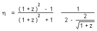
They are similar for small values of z.
- THE QUASAR PROBLEM:
...Quasars currently correspond to z values ranging from 0.13 to 4. The diameters of quasars are estimated from their fluctuation period T. We obtain a maximum diameter cT. Compared to the standard approach, this model gives larger values, because c was larger in earlier epochs.
...The volumetric power is referred to the size of galaxies. Let P_QSO be the absolute power emitted by a quasar and P_G the absolute power emitted by a galaxy. The relative power density of the QSO, compared to a galaxy, is:
(41)
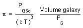
...But in our model, galaxies are no longer constant in size. They grow with time. Suppose the quasar is embedded in a galaxy. The size of this galaxy will grow as (1 + z). Thus, our correction factor, compared to standard values for power density, will involve three effects:
-
Change in distance (they are slightly closer).
-
Change in diameter (due to the variation of c).
-
Change in galaxy size.
Given P_QSO and P_G, the coefficient (57) becomes p' = p x with:
(42)
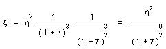
that is:
(43)
| z | h | x | |
|---|---|---|---|
| 0 | 1 | 1 | |
| 0.13 | 1.025 | 0.606 | The closest quasar |
| 0.2 | 1.03 | 0.467 | |
| 0.5 | 1.048 | 0.177 | |
| 1 | 1.024 | 0.0463 | |
| 1.5 | 0.985 | 0.0157 | |
| 2 | 0.946 | 0.0063 | |
| 2.5 | 0.912 | 0.00296 | |
| 3 | 0.882 | 0.00152 | |
| 3.5 | 0.856 | 0.000842 | |
| 4 | 0.834 | 0.0005 | The most distant quasar |
| 5 | 0.8 | 0.000201 | |
| 6 | 0.771 | 0.0001 | |
| 7 | 0.75 | 0.0000485 | |
| 8 | 0.731 | 0.0000275 | |
| 9 | 0.71 | 0.0000162 | |
| 10 | 0.7 | 0.0000102 |
...We see that this correction reduces the absolute magnitude of the observed quasar, and that this correction increases with z. Thus, if this model were correct, the classical model would have greatly overestimated the volumetric power density of quasars. Furthermore, the observed increase in the absolute magnitude of quasars could be due to the secular change in c.
Classically, the extent of galaxies is related to the Jeans length, but the model provides no available information about the sizes of emitting objects like stars or quasars. It depends on the energy emission process. Since we have not defined a possible gauge relation for the fusion coefficients, we do not yet have an available model. In any case, quasars could grow with time, like galaxies, and observations tend to support this hypothesis, which will be examined in more detail in the next paper devoted to the detailed interaction of the model and available observations.
- ASSOCIATED GAUGE RELATIONS.
...The ionization energy of hydrogen obeys: Eᵢ = 1/2 α² mₑc², where α is the fine-structure constant and mₑ the electron mass. We assumed that Eᵢ ∝ Rᵍ with g = 1, in order to fit the classical model, see (25), (33), and (35). Introduce the electron-proton mass ratio δ = mₑ/mₚ. According to the first paper [1], mₚ ∝ mₙ ∝ m ∝ R. Thus, mc² is an absolute constant. Then:
(44)

...The fine-structure constant α and the electron-proton mass ratio δ cannot be kept constant together. We will consider two possibilities;
9.1) Let us take δ ∝ constant. Then:
(45)
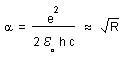
Introducing the gauge relations for h and c, we get: e²/ε₀ ∝ R³/² and the electromagnetic force F_em = e²/4πε₀R² ∝ R⁻¹/². Then:
(46)
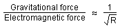
which is similar to an old idea of Dirac [4, 5].
Let us compute the