광속이 변하는 우주모형
광속이 변하는 측정 우주모형. QSO 관측 데이터와의 비교.
장피에르 피에트와 모리스 비톤 (우주천문학 연구소. 시폰 거리. 13012. 마르세유)
현대 물리학 편지 A, 제4권, 제23호 (1989) 2201-2210
요약 :
...이전 논문에서의 측정 불변성에 대한 보충 내용 이후, 우리는 최근에 발표된 134개의 QSO에 대한 데이터를 비교하였다. 이 데이터는 각각의 각도 크기와 루프의 곡률을 포함하고 있으며, 이는 우리가 새롭게 제안한 측정 우주모형 또는 일반적으로 받아들여지는 프리드만 모형(q₀ = 1/2)에서 기대되는 것과 비교된다. 새롭게 제안된 측정 모형이 적색편이에 따른 각도 크기 분포 및 곡률에 대해 더 나은 적합성을 보여준다는 것이 입증되었다. 이는 제트 형성에 관여하는 메커니즘에 대한 단순한 가정에 기반한다.
- 서론
...참조문헌 [1] 및 [2]에서, 이하 논문 I 및 논문 II로 지칭한다. 우리는 이전에 모든 물리 상수를 자유롭게 만든 우주모형을 개발하였다. 따라서 이러한 상수들을 편리하게 연결하기 위해 새로운 물리 법칙, 즉 측정 법칙을 도입해야 했다:
c(광속), G(중력), h(플랑크 상수), mₑ(전자 질량), mₚ, mₙ(양성자 및 중성자 질량). 먼저 일반 상대성 이론이 G와 c의 절대적인 일정성을 요구하지 않으며, 오직 G/c²(장 방정식의 아인슈타인 상수)의 절대적인 일정성만 요구한다는 것이 입증되었다. 이는 첫 번째 연결 관계를 제공하였다. 다른 관계는 기하학적 고려에서 나왔다: 우리는 줄리안 길이, 슈바르츠실트 길이 및 콤판 길이가 스케일 파라미터 R(t)의 변화를 따르는 것으로 가정하였다.
이 새로운 물리 법칙을 결합하여 다음 관계를 얻었다: (1)
(2)
mₚ = mₙ (핵자 질량) » R
(3)
h » R³/²
(4)
G » 1/R
(5)
V (속도) » R⁻¹/²
(6)
ρ » 1/R²
또한, 우리는 음의 곡률을 가진 단일 우주모형을 찾았으며, 이는 광자 또는 물질 또는 둘의 혼합으로 채워져 있으며, 비영인 압력을 가진다. 이 모형은 오직 하나의 법칙을 따르며: (7a)
...논문 II에서, 우리는 장기적인 플랑크 상수의 변화(시간에 비례함)에 의해 유도된 허블의 법칙을 재확인하였다. 이는 팽창 과정이 아닌 것이었다. 이 일정 에너지 모델에서, 기하학적 고려에 따라 특정 에너지(이온화 에너지 등)가 R(t)와 같이 변화하였다. 이는 전자기학에 적용된 추가적인 측정 관계와 일치하였다. 이후, 적색편이 데이터를 통해 광원의 거리를 도출할 수 있었다. 이 거리는 중간적인 z 값에서 일반적인 프리드만 모형(q₀ = 1/2)에서 도출된 값과 거의 같았다. 왜냐하면 비율:
(7b)
은 z ≤ 2에서 5% 이내로 단위에 가까웠기 때문이다.
- 측정 불변성에 대한 짧은 보충
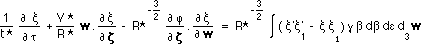
...논문 I, 5절에서, 우리는 몇 가지 기본 방정식(Vlasov, 슈뢰딩거, 맥스웰)이 제안된 측정 관계에 불변임을 보여주었다. 보스만 충돌 연산자가 또한 불변임을 보이자.
이 방정식을 쓰자. (8)
...f는 속도 분포 함수, g는 충돌 시 두 입자의 상대 속도, b는 길이(충격 파라미터), e는 각도이다. 차원 없는 변수를 도입하자. (9)
t = t* t ; f = f* x ; V = V* w ; g = V* g ; r = R* z
Y = (Gm/R*) j ; b = R* b
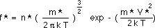
특성적인 속도 분포 함수는: (10)
...논문 I에서 정의된 측정 관계에 따라, Gm/R는 1/R와 같이 변한다. V는 1/R¹/²와 같이 변한다. m는 R와 같이 변한다( mV²는 일정). 에너지 kT는 일정하다. 요약하면 f * » R*⁻³/²이며, 따라서: (11)
...이러한 차원 분석은 각각 1/t*, V*/R* = 1/R³/², 1/R³/²과 같이 변하는 항을 제공한다. 이는 다시:
(12)
R* » t*²/³
를 의미하며, 이는 보스만 연산자의 불변성을 의미한다.
- 관측 검증
...이 짧은 주석 이후, 우리는 바르텔과 마일리[3, 이하 BM]가 최근에 발표한 134개의 QSO에 대한 데이터와 다양한 모델을 비교하자. 이들은 먼 DSO가 가까운 것보다 더 작은 각도 크기, 더 큰 곡률 및 더 높은 광도를 가진다고 보여주었다. 그러나 우리는 여기서 주어진 내재적 파워에 대해 논의하지 않을 것이며, 상대론적 제트를 생성하는 물리적 메커니즘은 여전히 명확하지 않기 때문이다.
...우주선의 각도 크기와 곡률에 대해 상황은 보다 단순하다. 이 두 경우 모두 기하학적 성질이 주로 작용한다. 그러나 우리는 다양한 체계적 효과가 작용할 수 있음을 간과할 수 없으며, BM이 제시한 세부 메커니즘에 대한 논의를 참조한다. 요약하자면:
-
은하간 매질(MIG)과의 상호작용은 초기에 정렬된 제트를 매우 효과적으로 방해하여, 넓고 흐트러진 루프를 형성한다. 만약 이러한 효과가 특정 적색편이에서 각도 크기 분포에 중대한 영향을 미친다면, BM은 먼 적색편이에서 관찰된 루프의 더 큰 곡률을 설명하기 위해 더 복잡한 메커니즘을 제안하였다.
-
위에서 언급된 모든 기본 메커니즘에서 가능한 진화적 효과, 심지어 아직 식별되지 않은 측정 과정 포함.
-
마를미스트 효과와 같은 관측적 편향으로 인해 먼 QSO의 각도 크기가 과소평가된다.
...이 논문에서 이러한 잠재적 효과가 데이터에서 주요하지 않다고 가정하자. 즉, 적색편이에 따른 각도 크기 및 곡률 분포는 다양한 우주모형을 구별하는 좋은 테스트로 간주할 수 있으며, 새로운 측정 모델이 이러한 분포에 더 나은 적합성을 보인다는 것을 보이자.
3a. 각도 크기.
...은하계 외부 물체의 각도 크기는 종종 우주모형에 대한 강력한 테스트로 간주되었다. 1은 발사 시기, 2는 수신 시기를 나타낸다. 광선은 시간 t₁에서 원천의 끝에서 방출되어 직선 경로를 따르므로, 현재 관측자는 각도 크기 f를 보존한다. 따라서 어떤 모델이든 다음과 같이 기술할 수 있다:
(13)
여기서 D(t₁)는 원천의 선형 직경, d(t₁)는 거리이다.
일반적인 프리드만 모델(q₀ = 1/2, 유명한 아인슈타인-데시터 모델)에서:
D(t₁) = D constant
R(t₁) = R(t₂) / (1 + z)
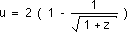
d(t₁) = R(t₁) u, 여기서:
(14)
그러므로 적색편이에 따른 각도 크기:
(15)
는 z = 1.25에서 최소값을 가지며, z와 함께 선형적으로 증가한다.
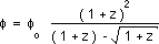
새로운 측정 모델에서는:
D(t₁) = D(t₂)/(1+z),
R(t₁) = R(t₂)/(1+z)
d(t₁) = R(t₁) u, 하지만:
(16)
각도 크기는:
(17)
z가 무한대로 갈수록 f는 일정해지며, 이는 데이터와 정성적으로 일치한다.
(18)
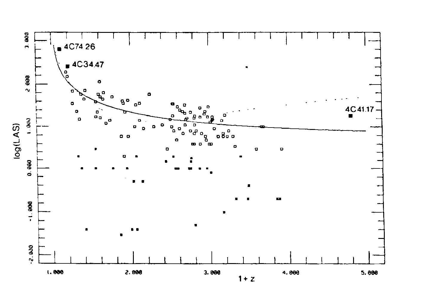
그림 18: 95개의 "T", "D1" 및 "D2" 형태의 확장된 원천(사각형) 및 33개의 "SSC" 형태의 밀집 원천(별표)에 대한 적색편이에 따른 최대 각도 크기(LAS, 초각 단위)를 로그 스케일로 표시한 것. 두 곡선은 본 논문에서 확장된 원천에 대해 얻은 측정 모델(실선) 및 아인슈타인-데시터 모델(점선)의 적합성을 나타낸다. 4C41.17은 현재 알려진 가장 먼 은하이며, 4C74.26는 퀀자와 연결된 가장 큰 라디오 원천이다.
...두 모델이 데이터에 얼마나 잘 적합하는지를 정량적으로 비교하기 위해, f = f₀f(z)로 쓰자. 여기서 f(z)는 각 모델이 위에서 예측한 특성 함수이다. "최대 각도 크기" [BM 이후 LAS] 데이터와 f(z) 사이에 선형 회귀 분석이 수행되었다. 이는 전체 134개의 QSO 샘플 또는 "T" 또는 "D1" 형태를 가진 이중 루프 원천만을 선택한 83개의 축소 샘플에 대해 수행되었다. 이는 "SSC" 또는 "D2" 형태의 원천을 제외하여 밀집 및 확장 원천 간의 가능한 다른 특성을 테스트하기 위한 것이었다. 회귀 분석 결과는 다음과 같다. 모든 선형 계수 및 RMS 오차 바는 초각 단위로 표현된다:
- 아인슈타인-데시터 모델을 사용할 경우:
F = (28.8 ± 2.9) f(z) - (89.3 ± 20.1)
전체 샘플에 대해, 그리고
F = (31.3 ± 3.3) f(z) - (90.5 ± 20.8)
축소 샘플에 대해.
- 측정 모델을 사용할 경우:
F = (21.5 ± 2.11) f(z) - (19.1 ± 19.6)
전체 샘플에 대해, 그리고:
F = (24.3 ± 2.3) f(z) - (17.3 ± 19.8)
축소 샘플에 대해.
...새로운 측정 모델이 데이터에 더 나은 적합성을 보인다는 것이 분명하다. 샘플이 무엇이든, 이 모델이 내포하는 중간 상수 항은 통계적으로 약간 유의미하며, 따라서 기대되는 0 값이 매우 가능하다. 반면, 일반적인 모델에서는 샘플이 무엇이든, 상수 항이 통계적으로 매우 유의미하며, 그 큰 음의 값은 이론적으로 받아들일 수 없으며, 위에서 언급된 강한 체계적 효과가 데이터에 작용하고 있다고 가정하지 않는 한이다.
3b. 곡률.
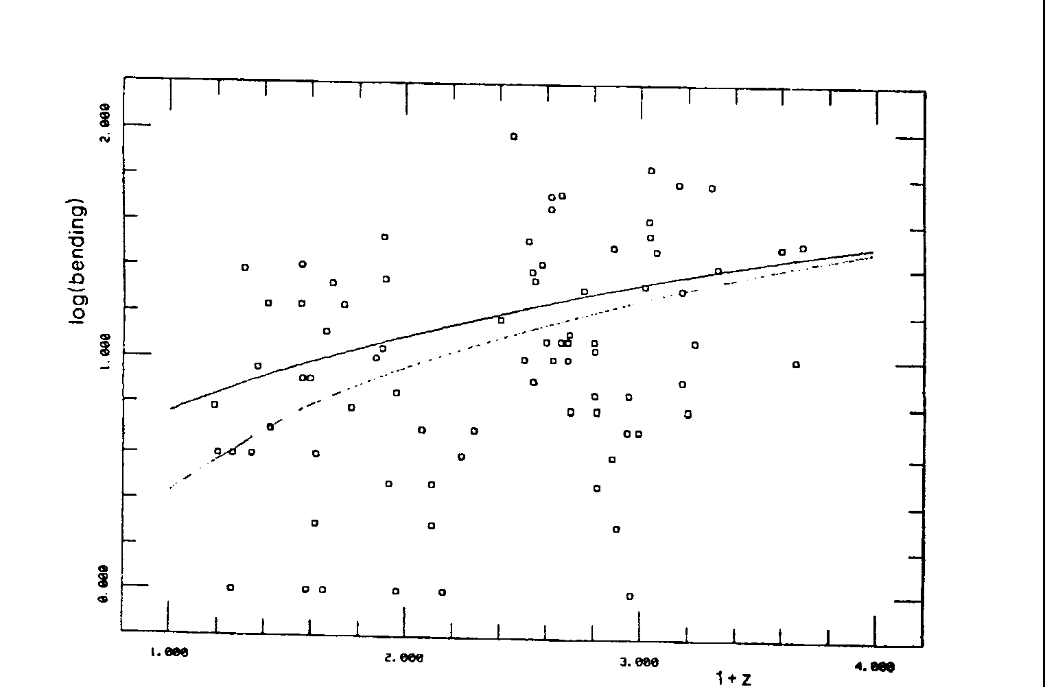
...BM이 강조한 먼 QSO의 더 곡률 있는, 더 왜곡된 외관이 새로운 측정 모델로 설명될 수 있음을 보이자. 이는 다양한 체계적 효과로 인한 결과가 아니라는 조건 하에 가능하다. 새로운 모델에서는 우주적 측정 과정 동안 모든 에너지가 보존된다고 가정하므로, QSO의 중심의 회전 에너지 보존을 포함할 수 있다: (19)
m » R, I » R³ 및 W » R⁻³/² W » 1/t » (1 + z)³/², 이는 BM이 축소 샘플에 대해 수행한 1차원 하한 법칙 적합과 흥미롭게 일치한다(곡률은 이 경우에만 정의됨). 즉:
(20)
그림 21: "T" 및 "D1" 형태의 83개 확장 원천에 대한 적색편이에 따른 곡률(도 단위)을 로그 스케일로 표시한 것. 이 곡률은 이 경우에만 정의된다. 실선은 측정 모델의 적합성을 나타내며, 이는 과거의 각속도가 더 높았음을 나타낸다. 점선은 바르텔과 마일리(BM)의 거듭제곱 법칙 적합을 나타낸다.
...이제, 최근 그레이버[5]의 분석을 참조하여 QSO의 중심 엔진의 성질과 그 엄청난 에너지 생산률에 대해 간단히 설명하자. 만약 (i) 플라즈마 덩어리가 QSO의 중심 엔진에서 지속적으로 또는 비지속적으로 자기 이중극 축을 따라 빠르게 방출된다는 사실을 받아들이고, (ii) 이 축이 일반적으로 각운동량 축과 일치하지 않는다는 사실을 받아들인다면, 우리는 회전하는 "정원 스프링클러"와 유사한 모델을 마주하게 된다. 이 경우, 제트는 스프링클러의 회전에 따라 아르키메데스 나선과 유사한 형태로 휘어진다. 이 상호작용이 은하간 매질(IGM)과 무시할 수 있을 정도로 작을 때까지이다. 이 상호작용이 중심에서 일정 거리 이상에서 의미 있게 되면, 제트는 그 지점에서 확장이 멈추며, 이로 인해 곡률이 증가한다. QSO 주변의 IGM 밀도가 구형으로 분포할 이유가 없으므로, 이러한 상호작용은 제트의 자주 발생하는 비대칭성과 전체 곡률에 대한 무작위 효과를 설명할 수 있다. 이는 BM이 논의한 바와 같다.
...결과적으로, QSO의 적색편이가 클수록 우주적 측정 과정으로 인해 각속도가 커지며, 따라서 제트의 곡률도 커진다.
- 결론.
...우리는 최근에 134개의 라디오 QSO에 대한 각도 크기 및 적색편이에 따른 곡률 분포에서 나타난 특정 특징에 집중하였다. 흥미롭게도, 우리는 "변하는 상수"를 가진 측정 모델이 일반적인 아인슈타인-데시터 모델보다 이러한 분포에 더 나은 적합성을 보인다는 것을 발견하였다. 이는 (i) 관측된 추세(먼 QSO의 더 작은 각도 크기 및 더 큰 곡률)가 미래 관측을 통해 확인되어야 하며, (ii) 이러한 추세가 다양한 효과나 오류에 의해 지배되지 않아야 하며, (iii) 일부 메커니즘에 대한 단순 가정이 사실이어야 한다는 조건 하에 가능하다. 또한, 측정 모델이 관측된 추세를 더 잘 이해할 수 있는지 여부를 이해하기 위해 이러한 원천의 내재적 파워에 대한 추가 조사가 필요하다. 즉, 먼 QSO의 광도가 가까운 QSO보다 훨씬 크다는 것이다.
- 참고문헌.
[1] J.P. PETIT : 광속이 변하는 우주모형의 해석. 현대 물리학 편지 A, 제3권, 제16호, 1988년 11월
[2] J.P. PETIT : 광속이 변하는 우주모형. 적색편이의 해석. 현대 물리학 편지 A, 제3권, 제18호, 1988년 12월.
[3] P.D. BARTHEL & G. K. MILEY. 퀀자에서의 라디오 구조의 진화 : 원시 은하의 새로운 탐지기? - Nature, 제333권, 1988년 5월 26일.
[4] M.L. NORMAN, J.O. BURNS 및 M.E. SULKANEN : 주변 매질의 충격에 의해 은하 라디오 제트의 방해, Nature 335 (1988) 146.
[5] H.D. GREYBER : 우주에서 강한 자기장의 중요성, Comments Astrophys. 13 (1989) 201.


원본(영어)
cosmological model with variable light velocity
**Gauge cosmological model with variable light velocity. Comparizon with QSO observational data. **
Jean-Pierre Petit and Maurice Viton (Laboratoire d'Astronomie Spatiale. Traverse du Siphon.13012. Marseille)
Modern Physics Letters A Vol.4 , n°23 (1989) pp. 2201-2210
ABSTRACT :
...After a complement to previous papers on the gauge invariance of the Boltzmann collisional operator, we compare a recent homogeneous set of data on radio-QSOs, including angular sizes and bending of lobes, with what is expected from either our new cosmological gauge model or the most commonly accepted Friedman model with qo = 1/2 . It is shown that the new gauge model provides a much better fit to the angular size distribution vs. redshift and similarly to the bending, thanks to crude hypothesis on the mechanisms involved with the formation of jets.
- INTRODUCTION
...In references [1] and [2] , hereafter paper I and paper II respectively, we have previously developped a cosmological model in which all the so called constants of physics were made free, so that we had to introduce new physical laws, gauge laws, in order to link conveniently these constants :
c (velocity of light), G (gravitation), h (Planck's constant), me (electron mass), mp, mn (proton and neutron mass ). It was shown at first that the general relativity theory does not require the absolute constancy of G and c, but only the absolute constancy of the ratio G/c2 (Einstein's constant of the field equation). This brought the first linking relation. The other came from geometric considerations : we assumed that the characteristic lengths like Jeans length, Schwarzschild length and Compton length followed the variation of the scale parameter R(t).
Combining these new physical laws we got the following relations : (1)
(2)
mp = mn ( nucleon's mass ) » R
(3)
h » R3/2
(4)
G » 1/R
(5)
V ( velocity ) » R-1/2
(6)
r » 1/R2
In addition we found a single cosmic model, with negative curvature, indifferently filled by photons or matter or a mixture of the two, with non zero pressure, and obeying the single law : (7a)
...In the paper II we refound the Hubble's law, due to the secular variation of the Planck constant (which was found to vary like t) and not to the expansion process. In this constant energy model, geometrical considerations made some characteristic energies like the ionization energy to vary like R(t), and it was found to be consistent with additional gauge relations applying to electromagnetism. Then it appeared possible to derive the distances of light sources from the red shift data. They were found to be quite close, for moderate z values, to the classical values derived from a Friedman model with qo = 1/2 , since the ratio :
(7b)
remains close to unity within 5 percent for z £ 2 .
- A SHORT COMPLEMENT ABOUT THE GAUGE INVARIANCE
...In the paper I, section 5, we had shown that some fundamental equations (Vlasov, Schrödinger, Maxwell) were invariant under the suggested gauge relations. Let us show that the Boltzmann collision operator is invariant to.
Writing this equation. (8)
...f is the velocity distribution function, g is the relative velocity of two particles in an encounter, b is a length (impact parameter), e an angle. Introduce adimensional variables, through : (9)
t = t* t ; f = f* x ; V = V* w ; g = V* g ; r = R* z
Y = (Gm/R*) j ; b = R* b
The characteristic velocity distribution function is : (10)
...Following the gauge relations as defined in paper I , Gm/R* varies like 1/R*. V* varies like 1/R1/2. m varies like R* (mV2 is constant). The energy k T is constant. To sum up f * » R*-3/2, and hence : (11)
...Such a dimensional analysis gives terms varying respectively like 1/t*, V*/R* = 1/R3/2 , 1/R3/2 , which implies again : (12)
R* » t* 2/3
and hence the invariance of the Boltzmann operator.
- OBSERVATIONAL TESTS.
...After this short parenthesis, let us turn to a comparison of various models with the radio data on 134 QSOs recently published by Barthel and Miley [ 3, hereafter BM] , in which they show that distant DSOs have smaller angular sizes, larger bendings and higher luminosities than those nearby. Note however that we do not intend to discuss the given intrinsic powers here, since the physical mechanisms involved in the generation of relativistic jets are not yet clearly understood.
...The situation is appearently simpler concerning the angular size and bending of radiosources, since geometric properties are mainly concerned a priori in both cases, though we cannot ignore that important systematic effects might be at work and we adress the reader to the related comprehensive discussion of BM on the detailed mechanisms involved. In short :
-
interaction with the intergalactic medium (IGM) can disrupt very efficiently the initially collimated jets, resulting into the formation of large, turbulent lobes (4) of lesser extension : if it is clear that such effects can modify significantly the angular size distribution at a given redshift, more complicated mechanisms have been invoked by BM to explain the stronger bending of lobes observed at large redshifts.
-
possible evolutionary effects in all the elementary mechanisms implicated above, including gauge processes not yet identified.
-
observational bias such as the well-known Malmquist's, introducing an underestimate of angular sizes for distant QSOs.
...Now, let us suppose in this paper that such potential effects are not dominant in the data, i.e. that the distribution of angular size and bending vs. redshifts may be considered as good tests for discriminating between different cosmological models and show that the new gauge model provides better fits to these distributions than do the conventional models.
3a The angular size.
...The angular size of extragalactic objects has often be considered as a powerfull test for cosmological models. So, let the subscript 1 refer to the emission epoch and subscript 2 to the reception epoch : since the light emited by the edges of a source at time t1 follows radial pathes, the angular size f is conserved for a present observer, so that we can write classically, whatever the model :
(13)
where D(t1) is the linear diameter of the source and d(t1) its metric distance.
In the classical Friedman model with qO = 1/2 ( the so called Einstein-de-Sitter's )
D(t1) = D constant
R (t1) = R (t2) / ( 1 + z )
and d(t1) = R (t1) u where :
(14)
and hence some kind of a paradox arises since the angular size obeys :
(15)
This function has a minimum for z = 1.25 , and then it tends to grow linearly with z .
Now, with the new gauge model we have
D(t1) = D(t2)/(1+z) ,
R(t1) = R(t2) / ( 1 + z )
and d(t1) = R (t1) u also
but with :
(16)
and the angular size obeys :
(17)
When z tends to infinity, f tends to a constant, a readily different behaviour and in qualitative agreement with the data.
(18)
Fig 18 : The largest angular size (LAS, in arcsecond), on a logarithmic scale versus redshift for the 95 extended sources with "T", "D1" and "D2" morphologies (squares) and the 33 compact sources with "SSC" morphologiy (asterisks). The two curves represent the fits of the gauge model (continuous line) and the Einstein-De Sitter model (dotted line) derived for extended sources in this paper. Three additional radio-sources of very large extent are shown for comparison. 4C41.17 being the farthest galaxy presently known, 4C74.26 the largest radio-source associated with a quasar.
...In order to compare quantitatively how both models fit the data, let us write f = fof(z) where f(z) is a characteristic function as predicted above by each model. Linear regressions have been performed between f(z) and the "largest angular size" [ LAS after BM ) data, either for their complete sample of 134 QSOs, or for a reduced sample of 83 QSOs in which only two-sided lobes sources were selected, i.e. those with the "T" or "D1" morphologies defined by BM, thus excluding the steep spectrum core or "SSC" and the one-sided lobe or "D2" sources, so as to test for possibly different properties of compact and extended sources. The results of the regressions were as follows, all the given linear coefficients and their rms errors bars being in arc second units :
- with the Einstein-de-Sitter model :
F = ( 28.8 ± 2.9 ) f(z) - ( 89.3 ± 20.1 )
for the complete sample, and
F = ( 31.3 ± 3.3 ) f(z) - ( 90.5 ± 20.8 )
For the reduced sample.
- with the gauge model :
F = ( 21.5 ± 2.11 ) f(z) - ( 19.1 ± 19.6 )
for the complete sample, and :
F = ( 24.3 ± 2.3 ) f(z) - ( 17.3 ± 19.8 )
for the reduced sample.
...It is clear that the new gauge model provides a fairly better fit to the data since whatever the sample, the moderate constant term it implies is marginally significant from a statistical point of view and hence the (expected) zero value is highly probable. The situation is quite opposite with the conventional model, here also whatever the sample, since the constant term is highly significant from a statistical point of view and its large, negative value is unacceptable on theoretical grounds, unless one supposes that very strong systematic effects as those suspected above are at work in the data.
3b. The bending.
...Let us show also that the more bent, distorted appearence of distant QSOs pointed out by BM may be curiously explained by the new gauge model, providing here again that is not an artefact resulting from various systematic effects. Since in the new model it is assumed that all the energies are conserved during the cosmic gauge process, we can include the conservation of the rotational energy of the QSO core emitting the jets : (19)
As m » R , I » R3 and W» R-3/2 W » 1/t » ( 1 + z )3/2, in curious agreement with the one-dimensional lower law fit performed by BM on the reduced sample ( since the bending is only defined in this latter case ), that is :
(20)
Fig 21: The bending (in degree) on a logarithmic scale versus redshift for the 83 extended sources with "T" and "D1" morphologies only, for which it is defined. The continuous curve corresponds to the fit of the gauge model, indicating that angular speeds where higter in the past, while the dotted line represents the power law fit of Barthel and Miley (BM)
...Now let us suggest a crude explanation, refering to the recent analysis of Greyber [5) on the nature of the central engines in QSOs responsible for their tremendous energy production rates : if we accept the figure (i) that the plasma blobs are ejected at high velocities from the central engine, continuously or not, along the magnetic dipole axis of the QSOs and (ii) that this latter is not generally coincident with their angular momentum axis, then we are faced with a model similar to a rotating "garden sprinkler", in which the jets will bend into some kind of a spiral of Archimedes, as long as the interaction with the IGM remains neglectible. And even if this interaction becomes significant at some distance from the nucleus, the jets will stop to expand there, resulting into an increased bending. Since there is no reason why the IGM density would be spherically distributed around QSOs, such interactions could account for the frequently assymetries in their jets together with random effects on the overall bending, as it has been discussed by BM.
...As a consequence, the higher the redshift of the QSO, the higher its angular velocity because of the cosmic gauge process and hence the larger the bending of its jets.
- CONCLUSION.
...We have focussed on specific features recently evidenced in the distribution of angular sizes and bending vs. redshift for an homogeneous set of 134 radio-QSOs. We found interestingly that our gauge model with "variable constants" provides better fits to these distributions than the conventional Einstein-de-Sitter model, providing (i) that the observed trends (smaller angular size and larger bending of distant QSOs) will be confirmed by future observations, (ii) that these trends are not dominated by various effects or artefacts, and (iii) that the crude assumptions wa made on some of the mechanisms involved are real. Also, further investigations on the intrinsic power of these sources are needed to understand if the gauge model provides a better understanding of the observed trends, i.e. that the luminosity of distant QSOs is much greater than for those nearby.
- REFERENCES.
[ 1] J.P.PETIT : Interpretation of cosmological model with variable light velocity. Modern Physics Letters A, Vol.3 n° 16 November 1988
[ 2] J.P.PETIT : Cosmological model with variable light velocity. The interpretation of red shifts. Modern Physics Letters A, Vol.3 , n° 18, December 1988.
[ 3] P.D.BARTHEL & G.KMILEY. Evolution of radio structure in quasars : a new probe of protogalaxies? - Nature Vol 333, 26 may 1988.
[ 4] M.L.NORMAN, J.O. BURNS and M.E. SULKANEN : Disruption of the galactic radio jets by the shocks in the ambient medium, Nature 335 (1988) 146.
[ 5] H.D.GREYBER : The importance of strong magnetic fields in the Universe, Comments Astrophys. 13 ( 1989 ) 201.