Kosmologisches Modell mit variabler Lichtgeschwindigkeit **
KOSMOLOGISCHES MODELL MIT VARIABLER LICHTGESCHWINDIGKEIT:
INTERPRETATION DER ROTVERSCHEIBUNGEN.
**
Jean-Pierre PETIT.
Observatoire de Marseille
Physics Letters A, Vol.3, Nr. 18, Dez. 1988, S. 1733
ZUSAMMENFASSUNG:
Das in Referenz [1] präsentierte Modell mit variablen c, G, h wird auf den Elektromagnetismus erweitert. Die Entropie erweist sich als proportional zu Log t und in einer Raum-Entropie-Darstellung ist die Metrik konform flach. Eine neue Eichbeziehung wird vorgeschlagen, die auf geometrischen Überlegungen basiert und einer Rydberg-Konstanten entspricht, die wie R variiert. Das Hubble-Gesetz gilt weiterhin. Das Alter des Universums bleibt unverändert, während seine Ausdehnung gleich der Hälfte des Mattig-Wertes gefunden wird. Eine vollständige Entschlüsselung der Rotverschiebung wird möglich. Die Entfernungen der Quellen sind sehr ähnlich. Die volumetrischen Leistungsdichten entfernter Quasare könnten stark überschätzt worden sein, während die Zunahme ihrer absoluten Helligkeit, wie sie aus der klassischen Theorie abgeleitet wird, auf die säkulare Variation von c zurückzuführen sein könnte. Unter der Annahme, dass das Massenverhältnis Elektron-Proton wie R variiert, erhält man eine Feinstrukturkonstante α, einen Bohrschen Radius und ein Verhältnis elektromagnetische Kraft zu Gravitationskraft, die sich wie absolute Konstanten verhalten.
1 - EINLEITUNG
...Mehrere Autoren haben versucht, Modelle mit zeitlich variierenden physikalischen Konstanten zu entwickeln [2, 3, 4, 5, 6, 7, 8, 9]. Keiner hat die Lichtgeschwindigkeit c in Frage gestellt, die stets als absolute Konstante betrachtet wurde. Wenn man die Form der Erhaltungsgleichungen beibehalten will, muss die Einstein-Konstante κ = - 8 π G / c² als absolute Konstante betrachtet werden. Unter diesen Bedingungen muss, wenn man die Lichtgeschwindigkeit c als absolute Konstante und eine variable Gravitationskonstante G beibehalten will, ein Quellterm zur Feldgleichung hinzugefügt werden, siehe Referenz [3]. Somit implizieren alle diese Theorien eine konstante Materieerzeugung.
...In einer früheren Arbeit [1] haben wir gezeigt, dass eine variable Lichtgeschwindigkeit zu einem konsistenten Modell führen kann, wenn G und die Planck-Konstante h geeigneten Eichbeziehungen folgen. Somit war die konstante Materieerzeugung nicht mehr notwendig. Die Erweiterung der Robertson-Walker-Metrik auf eine Konfiguration mit variabler Lichtgeschwindigkeit und ihre Einführung in die Feldgleichung ergab einen vollständigen Satz von Eichbeziehungen. Erinnern wir uns an die Hauptmerkmale des in [1] beschriebenen Modells:
(1)
(2) m (Teilchenmasse) ∝ R
(3) h (Planck-Konstante) ∝ R³/² ∝ t
(4) G (Gravitationskonstante) ∝ 1/R
(5) R (charakteristische Länge) ∝ t ²/³
(6) V (Geschwindigkeit eines freien Teilchens) ∝ R⁻¹/² ∝ c
(7) ρ (Massendichte) ∝ 1/R²
(8) mc² = Konstante
Im Folgenden folgt eine kurze Abschweifung zur Entropie.
- ZEIT ODER ENTROPIE?
Die relativistische Formulierung der Geschwindigkeitsverteilungsfunktion lautet:
(9)
wobei m die Ruhemasse, T die Temperatur, n die Teilchenzahldichte und K₂ eine Bessel-Funktion ist. Wenn b = (<v²>¹/²/c) << 1, erhält man die klassische Maxwell-Boltzmann-Geschwindigkeitsverteilungsfunktion: (10)
Berechnen wir die Entropie pro Baryon, definiert durch: (11)
wobei k die Boltzmann-Konstante ist. Wir haben n ∝ R⁻³, m ∝ R und R ∝ t²/³, T = Konstante (siehe Referenz [1]), sodass: (12)
Dann gilt: (13) s = k Log t + H( b )
Im Modell ist b eichinvariant, daher s ∝ Log t.
...In der klassischen Kosmologie ist das Universum isentropisch. Es könnte als etwas paradox empfunden werden, dass eine derart enorme Veränderung in der Zeit mit einer nahezu null Entropieänderung einhergeht. Im neuen Modell wächst die Entropie mit der Zeit. Beachten Sie, dass die BIG BANG-Singularität s = - ∞ entspricht.
Definieren wir nun die Entropie durch: (14) s = 3/2 k Log t
Kehren wir zur Robertson-Walker-Metrik zurück (15)
Wir erhalten: (16)
...In der Darstellung {Entropie, Raumvariablen} ist die Metrik konform flach. Aus kosmologischer Sicht könnte die Entropie (die andererseits unter Lorentz-Transformationen invariant ist) eine bessere Wahl als die Zeit sein. ...Darüber hinaus finden wir, wenn wir das Universum in einem Phasenraum (Position plus Geschwindigkeit) beschreiben, dass das charakteristische Hypervolumen R³c³ wie t variiert.
- DIE ROTVERSCHIEBUNG UND DIE ROBERTSON-WALKER-METRIK:
...Betrachten wir ein strahlendes Objekt, sagen wir einen Nebel N₁, der als Teilchen betrachtet werden kann. Nehmen wir an, sein Licht wird auf einem Nebel N₂ beobachtet, der im Ursprung der mitbewegten Koordinaten liegt. Der Nebel N₁ ist durch den Wert seines zeitunabhängigen Entfernungsparameters z gekennzeichnet, definiert durch die Beziehung:
(17)
Das zum Zeitpunkt t₁ emittierte Licht wird auf N₂ zu einem Zeitpunkt t₂ mit t₂ > t₁ beobachtet.
Der Abstand zwischen N₁ und N₂ ist R(t) dz und zeitabhängig, aber dz ist nicht zeitabhängig. Das Licht breitet sich auf einer nullgeodätischen Linie aus: (18)
ds² = (dx⁰)² - R² dz ² = 0
Betrachten wir das von N₁ bei einem entsprechenden Wert x⁰₁ + Δx⁰₁ des chronologischen Parameters emittierte Licht. Es wird bei x⁰₂ + Δx⁰₂ empfangen, wo es durch die Beziehung bestimmt wird: (19)
...Betrachten wir Δx⁰₁ als das Äquivalent der Periode eines physikalischen Phänomens, beispielsweise der Strahlungsemission, die auf N₁ stattfindet, und Δx⁰ als kurz im Vergleich zum Äquivalent der Laufzeit von N₁ nach N₂ (in Bezug auf den chronologischen Parameter x⁰). Das periodische Phänomen wird, von N₂ aus gesehen, eine „Periode“ Δx⁰₂ haben, sodass, gemäß der obigen Beziehung, die Zunahme des Integrals q null sein wird. Dies ergibt durch eine elementare Berechnung: (20)
Führen wir die kosmologische Zeit t ein, wie zuvor durch dx⁰ = c dt definiert, und schreiben R (x⁰₁) = R₁, R(x⁰₂) = R₂, c (x⁰₂) = c₂, c (x⁰₁) = c₁, so erhalten wir:
(21)

- DAS PROBLEM DES ELEKTROMAGNETISMUS:
...Wir können nicht mehr behaupten, dass die Energie Ei(t₁), die vom Atom zum Zeitpunkt t₁ emittiert wird, identisch mit der entsprechenden Emissionsenergie Ei(t₂) eines ähnlichen Atoms zum Zeitpunkt t₂ unter Laborbedingungen wäre. Die Lichtemission ist ein elektromagnetischer Prozess. Jeder weiß, dass die klassische Feldbeschreibung, die auf eine vierdimensionale Raumzeit angewendet wird, das elektromagnetische Phänomen nicht berücksichtigt. Um eine vollständige Beschreibung des Universums zu erhalten, sollten Gravitation und Elektromagnetismus in einen gemeinsamen geometrischen Rahmen eingebettet werden. Leider ist dies noch nicht zufriedenstellend geschehen, sodass unsere Arbeit etwas an innerer Kohärenz verliert. Nehmen wir beispielsweise an, die Rydberg-Konstante (Ionisierungsenergie des Wasserstoffs) gehorche einfach der folgenden hypothetischen Eichbeziehung: (22)
Ei ∝ Rg
(Beachten Sie, dass dies eine völlig willkürliche Annahme ist). Untersuchen wir die Konsequenzen dieser Annahme für die Entschlüsselung der Rotverschiebung. Später werden wir versuchen, sie mit möglichen Eichbeziehungen in Verbindung zu bringen.
- DAS PHÄNOMEN DER ROTVERSCHIEBUNG:
...In der klassischen Beschreibung ist die Rotverschiebung z auf den Doppler-Effekt zurückzuführen, plus einen zusätzlichen Effekt der speziellen Relativitätstheorie. Der Index 1 bezieht sich auf den Emitter und der Index 2 auf den Empfänger. Für eine gegebene spektroskopische Linie nennen wir E₁ = h₁ν₁₀ die Emissionsenergie und E₂ = h₂ν₂₀ die entsprechende Emissionsenergie unter heutigen Laborbedingungen für dieselbe Linie. Das Licht wird von einem ruhenden Atom bei der Frequenz ν₁ = ν₁₀ emittiert, was der Wellenlänge λ₁ = c₁/ν₁ = λ₁₀ entspricht.
ν₂ wird die gemessene Empfangsfrequenz sein, mit λ₂ = c₂/ν₂ und λ₂₀ = c₂/ν₂₀. Die Energie jedes Strahlungsprozesses folgt der allgemein angenommenen Eichgesetz (22).
Wir können die Rotverschiebung z definieren:
- Als das Verhältnis der Wellenlängen:
(23)
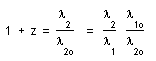
(24)
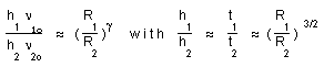
(a)
(b)
(c)
wir erhalten:
(25)

Beachten Sie, dass wir für g = 1 das klassische Modell wiederfinden.
- Als das Verhältnis der Frequenzen:
(26)
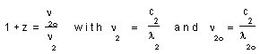
wir erhalten dasselbe Ergebnis.
- Als das Verhältnis der Energien.
(27)
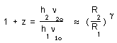
dasselbe. Die klassische Beziehung legt die Wahl g = 1 nahe.
- DAS HUBBLE-GESETZ UND DIE ROBERTSON-WALKER-METRIK:
Entwickeln wir die Funktion 1/R(t) in eine Reihe bezüglich
(28)

wir erhalten:
(29)
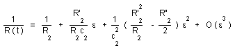
In R'² und R"² bezeichnet der Strich die Ableitung nach t. Insbesondere, in erster Ordnung:
(30)
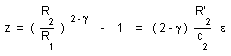
Dann entwickeln wir die folgenden Ausdrücke:
(31a)
(b)
(c)
Bezugnehmend auf die erste Ordnung:
(32)
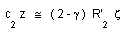
Als erste Näherung misst der Astronom d₂ ≈ R₂ z, sodass:
(33)
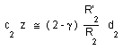

Dies ist nichts anderes als das Hubble-Rotverschiebungsgesetz, das auch in diesem Rahmen mit variabler Lichtgeschwindigkeit gilt. Aus der Messung von d₂, c₂ und z können wir die sogenannte Hubble-Konstante ableiten, das heißt das Alter des Universums.
Nehmen wir R = 3/2 c t (siehe Referenz [1]).
(34)

Das Alter des Universums entspricht:
(35)
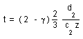
Ein Wert g = 1 ergibt den Wert des Standardmodells.
- DIE ROTVERSCHIEBUNG UND DIE ENTFRONUNGSENTSCHÄTZUNG:
Kehren wir zur Robertson-Walker-Metrik zurück, die liefert:
(36)
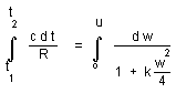
Im klassischen Ansatz nehmen wir das Einstein-de-Sitter-Modell (k = 0). Wir erhalten:
(37a)
Mit R = a t²/³ haben wir:
(b)
woraus
(38)

Wenn z klein ist: d₂ ∝ 3/2 ct₂ z
wenn z gegen unendlich strebt: d₂ strebt gegen 3 c t₂
Natürlich ergibt die Mattig-Formel dasselbe Ergebnis:
(39a)
(b)
(c)
Kehren wir zur Robertson-Walker-Metrik zurück, gemäß unserem Modell, mit k = - 1:
(d)
schreiben wir:
(e)
(f)
Sei:
(g)
Dann:
(h)
Für radiale Wege:
(i)
(j)
Log ( 1 + z ) = Arg th u
(k)
(l)
Wenn z gegen unendlich strebt, finden wir den Horizont (3/2)c₂t₂, der doppelt so klein ist wie der Standardwert 3 c₂t₂.
Beachten Sie, dass dies völlig ähnlich ist zum Gesetz, das vr/c (wobei vr die Radialgeschwindigkeit ist) in Abhängigkeit von z im Standardmodell angibt.
Vergleichen wir die Entfernungen, wie sie durch unser Modell und das Standardmodell gegeben sind.
(40)
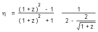
Sie sind für kleine z-Werte ähnlich.
- DAS PROBLEM DER QUASARE:
...Quasare entsprechen derzeit z-Werten von 0,13 bis 4. Die Durchmesser der Quasare werden aus ihrer Fluktuationsperiode T geschätzt. Wir erhalten einen maximalen Durchmesser cT. Im Vergleich zum Standardansatz liefert dieses Modell größere Werte, da c in früheren Zeiten größer war.
...Die volumetrische Leistung wird auf die Größe der Galaxien bezogen. Nennen wir P_QSO die absolute Leistung, die von einem Quasar emittiert wird, und P_G die absolute Leistung, die von einer Galaxie emittiert wird. Die relative Leistungsdichte des QSO im Vergleich zu einer Galaxie ist:
(41)
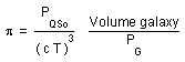
...Aber in unserem Modell sind die Galaxien nicht mehr konstant in ihrer Größe. Sie wachsen mit der Zeit. Nehmen wir an, der Quasar ist in eine Galaxie eingebettet. Die Größe dieser Galaxie wird wie (1 + z) wachsen. Somit wird unser Korrekturfaktor im Vergleich zu den Standardwerten für die Leistungsdichte drei Effekte beinhalten:
-
Änderung der Entfernung (sie sind etwas näher).
-
Änderung des Durchmessers (aufgrund der Variation von c).
-
Änderung der Galaxiengröße.
Gegeben P_QSO und P_G wird der Koeffizient (57) zu p' = p x mit:
(42)
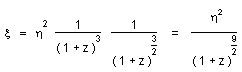
das heißt:
(43)
| z | h | x | |
|---|---|---|---|
| 0 | 1 | 1 | |
| 0,13 | 1,025 | 0,606 | Der nächste Quasar |
| 0,2 | 1,03 | 0,467 | |
| 0,5 | 1,048 | 0,177 | |
| 1 | 1,024 | 0,0463 | |
| 1,5 | 0,985 | 0,0157 | |
| 2 | 0,946 | 0,0063 | |
| 2,5 | 0,912 | 0,00296 | |
| 3 | 0,882 | 0,00152 | |
| 3,5 | 0,856 | 0,000842 | |
| 4 | 0,834 | 0,0005 | Der entfernteste Quasar |
| 5 | 0,8 | 0,000201 | |
| 6 | 0,771 | 0,0001 | |
| 7 | 0,75 | 0,0000485 | |
| 8 | 0,731 | 0,0000275 | |
| 9 | 0,71 | 0,0000162 | |
| 10 | 0,7 | 0,0000102 |
...Wir sehen, dass diese Korrektur die absolute Helligkeit des beobachteten Quasars reduziert und dass diese Korrektur mit z zunimmt. Somit hätte, wenn dieses Modell gut wäre, das klassische Modell die volumetrische Leistungsdichte der Quasare stark überschätzt. Darüber hinaus könnte die beobachtete Zunahme der absoluten Helligkeit der Quasare auf die säkulare Änderung von c zurückzuführen sein.
Klassisch ist die Ausdehnung der Galaxien mit der Jeans-Länge verbunden, aber das Modell liefert keine verfügbaren Informationen über die Größen von emittierenden Objekten wie Sternen oder Quasaren. Es hängt vom Energieemissionsprozess ab. Da wir keine mögliche Eichbeziehung für die Fusionskoeffizienten definiert haben, haben wir noch kein verfügbares Modell. Jedenfalls könnten die Quasare mit der Zeit wachsen, wie die Galaxien, und die Beobachtungen neigen dazu, diese Hypothese zu unterstützen, die im nächsten Artikel, der sich mit der detaillierten Wechselwirkung des Modells und der verfügbaren Beobachtungen befasst, genauer untersucht wird.
- ZUGEORDNETE EICHBEZIEHUNGEN.
...Die Ionisierungsenergie des Wasserstoffs gehorcht: Ei = 1/2 α² m_e c², wobei α die Feinstrukturkonstante und m_e die Masse des Elektrons ist. Wir haben angenommen, dass Ei ∝ Rg mit g = 1, um sich an das klassische Modell anzupassen, siehe (25), (33) und (35). Führen wir das Massenverhältnis Elektron-Proton δ = m_e/m_p ein. Gemäß dem ersten Artikel [1] gilt m_p ∝ m_n ∝ m ∝ R. Somit ist mc² eine absolute Konstante. Dann:
(44)

...Die Feinstrukturkonstante α und das Massenverhältnis Elektron-Proton δ können nicht gleichzeitig konstant gehalten werden. Wir werden zwei Möglichkeiten betrachten;
9.1) Nehmen wir zunächst δ ∝ Konstante. Dann:
(45)
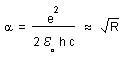
Durch Einführung der Eichbeziehungen für h und c erhalten wir: e²/ε₀ ∝ R³/² und die elektromagnetische Kraft F_em = e²/4πε₀R² ∝ R⁻¹/². Dann:
(46)
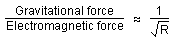
was einer alten Idee von Dirac ähnelt [4, 5].
Berechnen wir den
Originalversion (Englisch)
cosmological model with variable light velocity **
COSMOLOGICAL MODEL WITH VARIABLE LIGHT VELOCITY :
THE INTERPRETATION OF RED SHIFTS.
**
Jean-Pierre PETIT.
Observatoire de Marseille
Modern Physics Letters A, Vol.3 , n° 18, dec. 1988, p.1733
ABSTRACT :
cThe model with variable c, G, h presented in reference [1] is extended to electromagnetism. The entropy is found to vary like Log t and, in a space-entropy representation, the metric is conformally flat. A new gauge relation is suggested, based on geometrical considerations, which corresponds to a Rydberg constant varying like R. The Hubble's law still applies. The age of the universe is unchanged while its span is found to be half of the Mattig's value. The complete decoding of the red shift can be done. The distances of the sources are very similar. The large volumic power densities of distant quasars could have been greatly overestimated, while the increase of their absolute magnitude, as derived from the classical theory, could be due to the secular variation of c. Assuming the electron-proton mass ratio to vary like R we get a fine structure constant a, a Bohr radius and a ratio electromagnetic force to gravitational force which behave like absolute constants.
**1 - **INTRODUCTION
...Several authors tried to develop models with physical constants in time varying in time [2, 3, 4, 5, 6, 7, 8, 9] . None questionned the light velocity c, always considered an absolute constant. If one wants to save the form of the conservation equations, the Einstein's constant c = - 8 p G / c2 must be considered as an absolute constant. In such conditions if one wants to keep the light velocity c as an absolute c constant and a variable gravitational constant G, one must add a source term to the field equation, see reference [3] . Thus, all these theories imply a constant creation of matter.
...In a previous paper [1] we showed that a variable ligth-velocity could lead to a consistent model if both G and the Planck's constant h followed convenient gauge relations. Thus, the constant creation of matter was no longer necessary. The extension of the Robertson-Walker metric to a variable light velocity configuration and its introduction into the field equation gave a complete set of gauge relations. Let us recall the main features of the model described in [1] :
(1)
(2) m ( particle's mass ) » R
(3) h ( Planck'constant ) » R3/2 » t
(4) G ( Gravity constant ) » 1/R
(5) R ( Characteristic length ) » t 2/3
(6) V ( Velocity of a free particle ) » R-1/2 » c
(7) r ( mass density )» 1/R2
(8) mc2 = constant
The following is a short digression about entropy.
- TIME OR ENTROPY ?
The relativistic formulation of the velocity distribution function is :
(9)
where m is the rest mass, T the temperature, n the number of density and K2 a Bessel function. If b = (1/2/c) << 1 then we get the classical Maxwell-Boltzmann velocity distribution function : (10)
Let us compute the entropy per baryon, as defined by : (11)
where k is the Botzmann's constant. We have n » R-3 , m » R and R » t2/3, T = constant ( see reference [ 1] ) , such as : (12)
Then : (13) s = k Log t + H( b )
In the model b is gauge invariant such as s » Log t.
...In the classical cosmology the universe is isentropic. One could consider somewhat paradoxal that such enormous change in time goes with an almost zero entropy variation. In the new model the entropy grows with time. Notice that the BIG BANG singularity corresponds to s = - ¥ .
Let us define now the entropy through : (14) s = 3/2 k Log t
Let us return to the Robertson-Walker metric (15)
We get : (16)
...In the representation { entropy, space variables } the metric is conformally flat. From a cosmological point of view, the entropy (which on another hand is invariant with respect to the Lorentz transform ) could be a better choice than time. ...In addition, if we describe the universe in a phase space ( position plus velocity ) we find that the associated characteristic hypervolume R3c3 varies like t.
- THE RED SHIFT AND THE ROBERTSON-WALKER METRIC :
...Consider a radiating object, say a nebula N1, which could be considered as a particle. Suppose his light is observed on a nebula N2 placed at the origin of the co-moving coordinates. The nebula N1 is characterized by the value of its time-independent distant marker z, defined by the relation :
(17)
The light emited at time t1 is observed on N2 at a time t2 with t2 > t1 .
The distance between N1 and N2 is R(t) dz and is time-dependent but dz is not. Light travels on a nul geodesic : (18)
ds2 = (dx°)2 - R2 dz 2= o
Consider the light emited by N1 at a corresponding value x°1 + D x°1 of the chronological parameter. It will be received at x°2 + D x°2, where it will be determined through the relation : (19)
...Consider D x°1 as the equivalent of the period of some physical phenomenon, the emission of radiation for instance, taking place on N1 , and Dx° to be short compared to the equivalent of the travel time from N1 to N2 ( in term of chronological parameter x° ). The periodic phenomenon will appear, as seen from N2 , to have a "period" D x°2 which, from the above relation, will be such that the increment of the q integral will be zero. This, by elementary calculus, gives : (20)
Let us introduce the cosmic time t as defined before through dx° = c dt and write R (x°1) = R1 , R(x°2) = R2 , c (x°2) = c2 , c (x°1) = c1 , then we get :
(21)
- THE PROBLEM OF ELECTROMAGNETISM :
...Now we cannot assert that the energy Ei(t1), emitted by the atom at the time t1 would be identical to the corresponding emission energy Ei(t2) of a similar atom, at time t2, in lab's conditions. The light emission is an electromagnetic process. Everybody knows that the classical field description, applying to a four dimensional space time does not take in charge the electromagnetic phenomenon. To get a complete description of universe gravitation and electromagnetism should be imbedded in a common geometrical framework. Unfortunately it has not been done yet in a satisfactory way so that our work will now loose somewhat its self-consistency. . Suppose, for instance, that the Rydberg constant ( ionization energy of hydrogen ) would simply obey the following hypothetic gauge relationship : (22)
Ei » Rg
( Notice that this is a totally arbitrary assumption ). Let us explore the consequences of it on the red shift decoding. Later we will try to relate it to possible gauge relations.
- THE RED SHIFT PHENOMENON :
...In the classical description the red shift z is due to the Doppler effect, plus some special relativity additional effect. The indix 1 refers to the emitter and the indix 2 to the receiver. For a given specctroscopic line, call E1 = h1n1o the emission energy and E2 = h2n2o the corresponding emission energy in the today's lab's conditions, for the same line. The light is emitted by an atom at rest at the frequency n1 = n1o, corresponding to the wavelength l1 = c1/n1 = l1O.
n2 will be the mesured reception frequency, with l2 = c2/n2 and l2o = c2/n2o . The energy of any radiative process will follow the general assumed gauge law (22).
We can define the red shift z :
- As the ratio between the wavelengths :
(23)
(24)
(a)
(b)
(c)
then we get :
(25)
Notice that, for g = 1 we refind the classical model.
- As the ratio between the frequencies :
(26)
we get the same result.
- As the ratio between the energies.
(27)
same thing. The classical relation suggests the choice g = 1 .
- THE HUBBLE'S LAW AND THE ROBERTSON WALKER METRIC :
Let us expand the function 1/R(t) into a series with respect to
(28)
we get :
(29)
In R'2 and R"2 the prime denotes differentiation with respect to t. In particular , at the first order :
(30)
Next, expanding the following expressions :
(31a)
(b)
(c)
Refering to the first order :
(32)
As a first approximation the astronomer measures d2 @ R2 z, such as :
(33)
Which is nothing but the Hubble's red shift law, which still applies in this variable light velocity conditions. From mesurement of d2, c2 and z we can derive the so called Hubble's constant, i.e. the age of universe.
Take R = 3/2 c t ( see reference [ 1) ).
(34)
The age of universe corresponds to :
(35)
A g = 1 value gives the standard model value.
- THE RED SHIFT AND THE DISTANCE EVALUATION :
Let us return to the Robertson-Walker metric, which provides :
(36)
In the classical approach, take the Einstein-de Sitter model ( k = o ). We get :
(37a)
With R = a t2/3 we have :
(b)
whence
(38)
If z is weak : d2 » 3/2 ct2 z
if z tends to infinite : d2 tends to 3 c t2
Of course the Mattig's formula gives the same result :
(39a)
(b)
(c)
Let us return to the Robertson Walker metric, following our model, with k = - 1 :
(d)
write :
(e)
(f)
Let :
(g)
Then :
(h)
For radial pathes :
(i)
(j)
Log ( 1 + z ) = Arg th u
(k)
(l)
When z tends to infinite we refind the horizon (3/2)c2t2, which is twice smaller than the standard value 3 c2t2 .
Notice this is completely similar to the law giving vr/c ( where is the radial velocity ) as a function of z, ine the standard model.
Let us compare the distances, as given by our model and the standard model.
(40)
They are similar for weak z values.
- THE QUASARS PROBLEM :
...Quasars correspond presently to z values from 0.13 to 4 . The diameters of the quasars are estimated from their fluctuation period T. We get a maximum diameter cT. With respect to the standard approach this model gives larger values, for c was larger in the earlier time.
...The volumic power is refered to the size of the galaxies. Call PQSO the absolute power emited by a quasar and PG the absolute power emited by a galaxy. The relative power density of the QSO, with respect to a galaxy, is :
(41)
...But in our model the galaxies are no longer constant in size. They grow in time. Suppose the quasar is imbedded in a galaxy. The size of this galaxy will grow like ( 1+ z ). Such as our correcting term, with respect to the standard values for power density, will involve three effects :
-
Change for the distance ( they are a little bit closer ).
-
Change for the diameter ( due to the variation of c ).
-
Change of the galaxy's size.
Given PQSO and PG the coefficient (57) becomes p' = p x with :
(42)
i.e :
(43)
| z | h | x | |
|---|---|---|---|
| 0 | 1 | 1 | |
| 0,13 | 1.025 | 0,606 | The closest quasar |
| 0,2 | 1.03 | 0.467 | |
| 0.5 | 1.048 | 0.177 | |
| 1 | 1.024 | 0.0463 | |
| 1.5 | 0.985 | 0.0157 | |
| 2 | 0.946 | 0.0063 | |
| 2.5 | 0.912 | 0.00296 | |
| 3 | 0.882 | 0.00152 | |
| 3.5 | 0.856 | 0.000842 | |
| 4 | 0.834 | 0.0005 | The most distant quasar |
| 5 | 0.8 | 0.000201 | |
| 6 | 0.771 | 0.0001 | |
| 7 | 0.75 | 0.0000485 | |
| 8 | 0.731 | 0.0000275 | |
| 9 | 0.71 | 0.0000162 | |
| 10 | 0.7 | 0.0000102 |
...We see that this correction reduces the absolute magnitude of the observed quasar, and that this correction increases with z. Thus, would this model would be good, the classical model would have greatly overestimated the volumic power density of quasars. In addition the observed increase of absolute magnitude of quasars could be due to the secular change in c.
Classically the galaxies' span are related to the Jeans' length, but the model does not provide any avaible information about the sizes of some emitting objects like stars or quasars. It depends on the energy emission process. As we have not defined some possible gauge relation for the fusion coefficients we have no avaible model yet. Anyway the quasars could grow in time, like galaxies and the observations tend to support this hypothesis, that will be examined with more details in the next paper devoted to the detailed interaction of the model and avaible observations. .
- ASSOCIATED GAUGE RELATIONS.
...The ionization energy of hydrogen obeys : Ei = 1/2 a2 mec2, where a is the fine structure constant and me the mass of the electron. We have assumed that Ei » Rg with g = 1, in order to fit with the classical model, see (25), (33) and (35). Introduce the electron-proton mass ratio d = me/mp . According to the first paper [ 1] mp » mn » m » R. So that mc2 is an absolute constant. Then :
(44)
...The fine structure constant a and the electron-proton mass ratio d cannot be kept constant together. We shall consider two possibilities ;
9.1) Let us take first d » constant. Then :
(45)
Introducing the gauge relations for h and c we get : e2 /eo » R3/2 and the electromagnetic force Fem =e2 /4peoR2 » R-1/2. Then :
(46)
which is similar to an old idea of Dirac [ 4, 5] .
Let us compute the Bohr radius :
(47)
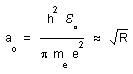
9.2) Now we take a » absolute constant. Then me » R2. and e2 /eo » R. The Compton length of the electron h/mec, the ratio gravitational force to the electromagnetic force and the Bohr radius become absolute constants.
...In the references [10] to [13] several authors study the possible variability of several quantities : a, a2(gp/ge)(me/mp) , me/mp ,where gp and ge are the gyromagnetic ratios of the proton and the electron. Following B.E.G. PAGEL [13] , we have :
Effect
Quantity Approximate 3
s
upper
limit to variation.
| Optical doublet splitting. | a | 3 % | | | | | | | | | | | |
Comparizon of optical and 21 cm redshifts. a 2 ( g p/ g e) (m e /m p) 10 -3
| Comparizon of hydrogen and metal redshifts. | d = | m | e | /m | p | 50% | | | | | | | |
...As a consequence we choose the second possibility, with a variable mass ratio. Notice that in both cases we get gp/ge » 1/R.
1O) CONCLUSION
...Here we tried to extend the model introduced in reference [1] to electromagnetism. A gauge law was suggested : we assumed the ionisation energy Ei ( Rydberg constant ) to vary like Rg. Local geometrical considerations recommand the value g = 1 , which takes account of the desonization process during the cosmic evolution. The distance of a radiative source, as derived from the Robertson Walker metric, gives results quite similar to the standard model'values, but this new model tends to reduce considerably the estimated density power of distant sources like quasars. In addition the increase of absolute magnitude in z, as derived from the classical model, could be due to the secular variation in c.
...With an electron-proton mass ratio d = me/mp which varies like R we get a fine structure constant a which behaves like an absolute constant.
REFERENCES :
[ 1] J.P.PETIT : An interpretation of cosmological model with variable light velocity. Modern Physics Letters A......
[ 2] E.A. MILNE : Kinematic Relativity Oxford 1948.
[ 3] F.HOYLE & J.V.NARLIKAR : Cosmological models in conformally invariant gravitational theory. Mon. Notices Roy. Astr. Soc. 1972 155 pp 3O5-325.
[ 4] P.A. DIRAC : 1937, Nature, **139,**323
[ 5] P.A. DIRAC : 1973 Proc. Roy. Soc. London , A333, 4O3
[ 6] V.CANUTO & J.LODENQUAI : Dirac cosmology, Ap.J. 211 : 342-356 1977 January 15.
[ 7] T.C.VAN FLANDERN : Is the gravitational constant changing ? Ap.J, 248 : 813-816
[ 8] A.JULG. Dirac's large numbers hypothesis and continuous creation. Ap.J. 271 : 9-1O 1983 August 1
[ 9] V.CANUTO & S.H. HSIEH : The 3 K blackbody radiation, Dirac's large numbers hypothesis, and scale-covariant cosmology. Ap.J., 224 : 3O2-307, 1978 September 1
[ 10] B.E.J.PAGEL : On the limits to past variability of the proton-electron mass ratio set by quasar absorbtion line redshifts. Mon. Not. astr. Soc. (1977), short communication, 81P-85P.
[ 11] A.M.WOLFE & R.L.BROWN & M.S.ROBERTS. Limits on the variation of fundamental atomic quantities over cosmic time scales. Physical Review Letters Vol 37, number 4, 26 July 1976.
[ 12] A.D.TUBBS & A.M.WOLFE : Evidence for large-scale uniformity of physical laws. A.P.J, 236 : L1O5-1O8, 198O March 15
[ 13] B.E.J.PAGEL. Implication of quasar spectroscopy for constancy of constants. Phil. Trans. R. Soc. Lond. 3 31O, 245-247 , 1983.