modelo cosmológico con velocidad de la luz variable

modelo cosmológico con velocidad de la luz variable

Modelo cosmológico de gauge con velocidad de la luz variable. Comparación con datos observacionales de QSO.

Jean-Pierre Petit y Maurice Viton (Laboratoire d'Astronomie Spatiale. Traverse du Siphon. 13012. Marsella)

Physics Letters A Vol. 4, n° 23 (1989) pp. 2201-2210

RESUMEN:

...Después de un complemento a artículos anteriores sobre la invariancia de gauge del operador de colisión de Boltzmann, comparamos un conjunto reciente y homogéneo de datos sobre QSOs radio, incluyendo los tamaños angulares y las curvaturas de los lóbulos, con lo que se espera a partir de nuestro nuevo modelo cosmológico de gauge, o del modelo de Friedmann más comúnmente aceptado con q₀ = 1/2. Se muestra que el nuevo modelo de gauge proporciona un mejor ajuste a la distribución de los tamaños angulares en función del corrimiento al rojo, así como a la curvatura, gracias a suposiciones simples sobre los mecanismos involucrados en la formación de los chorros.

1. INTRODUCCIÓN

...En las referencias [1] y [2], a continuación artículo I y artículo II respectivamente, previamente desarrollamos un modelo cosmológico en el cual todas las constantes llamadas de la física se convirtieron en libres, de modo que tuvimos que introducir nuevas leyes físicas, leyes de gauge, para relacionar convenientemente estas constantes:

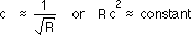
c (velocidad de la luz), G (gravedad), h (constante de Planck), mₑ (masa del electrón), mₚ, mₙ (masa del protón y del neutrón). Se mostró primero que la teoría de la relatividad general no exige la constancia absoluta de G y c, sino solamente la constancia absoluta del cociente G/c² (constante de Einstein de la ecuación del campo). Esto dio la primera relación de enlace. La otra vino de consideraciones geométricas: supusimos que las longitudes características como la longitud de Jeans, la longitud de Schwarzschild y la longitud de Compton seguían la variación del parámetro de escala R(t).

Combinando estas nuevas leyes físicas, obtuvimos las siguientes relaciones: (1)

(2)

mₚ = mₙ (masa del nucleón) » R

(3)

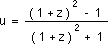
h » R³/²

(4)

G » 1/R

(5)

V (velocidad) » R⁻¹/²

(6)

ρ » 1/R²

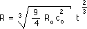
Además, encontramos un único modelo cosmológico con curvatura negativa, lleno indistintamente de fotones o de materia o de una mezcla de ambos, con presión no nula, y que obedece a la única ley: (7a)

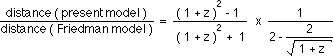
...En el artículo II, recuperamos la ley de Hubble, debido a la variación secular de la constante de Planck (que resultó variar como t) y no al proceso de expansión. En este modelo de energía constante, consideraciones geométricas hicieron variar ciertas energías características como la energía de ionización como R(t), y esto resultó coherente con relaciones de gauge adicionales aplicadas al electromagnetismo. Luego, resultó posible deducir las distancias de las fuentes luminosas a partir de los datos de corrimiento al rojo. Se revelaron bastante cercanas, para valores moderados de z, a los valores clásicos deducidos de un modelo de Friedmann con q₀ = 1/2, ya que el cociente:

(7b)

permanece cercano a la unidad dentro del 5 por ciento para z ≤ 2.

2. UN BREVE COMPLEMENTO SOBRE LA INVARIANCIA DE GAUGE

...En el artículo I, sección 5, mostramos que ciertas ecuaciones fundamentales (Vlasov, Schrödinger, Maxwell) eran invariantes bajo las relaciones de gauge propuestas. Mostremos que el operador de colisión de Boltzmann también lo es.

Escribamos esta ecuación. (8)

...f es la función de distribución de velocidades, g es la velocidad relativa de dos partículas durante un encuentro, b es una longitud (parámetro de impacto), e un ángulo. Introduzcamos variables sin dimensiones, mediante: (9)

t = t* t ; f = f* x ; V = V* w ; g = V* g ; r = R* z

Y = (Gm/R*) j ; b = R* b

La función de distribución de velocidades característica es: (10)

...Según las relaciones de gauge tal como están definidas en el artículo I, Gm/R* varía como 1/R*. V* varía como 1/R¹/². m varía como R* (mV² es constante). La energía kT es constante. En resumen f * » R*⁻³/², y por lo tanto: (11)

...Un análisis dimensional da términos que varían respectivamente como 1/t*, V*/R* = 1/R³/², 1/R³/², lo que implica nuevamente: (12)

R* » t*²/³

y por lo tanto la invariancia del operador de Boltzmann.

3. PRUEBAS OBSERVACIONALES.

...Después de esta breve pausa, pasemos a una comparación entre diversos modelos y los datos radio sobre 134 QSOs recientemente publicados por Barthel y Miley [3, a continuación BM], en los cuales muestran que los DSO lejos tienen tamaños angulares más pequeños, curvaturas más importantes y luminosidades más altas que los objetos cercanos. Sin embargo, notemos que no tenemos la intención de discutir aquí las potencias intrínsecas dadas, ya que los mecanismos físicos involucrados en la generación de los chorros relativistas no están aún claramente comprendidos.

...La situación parece aparentemente más simple en cuanto al tamaño angular y la curvatura de las fuentes radio, ya que las propiedades geométricas están principalmente en juego a priori en ambos casos, aunque no podamos ignorar que puedan haber efectos sistemáticos importantes en juego, y remitimos al lector a la discusión exhaustiva de BM sobre los mecanismos detallados involucrados. En resumen:

• la interacción con el medio interestelar (MIG) puede perturbar muy eficientemente los chorros inicialmente colimados, causando la formación de lóbulos grandes, turbios, de menor alcance: si aceptamos que tales efectos pueden modificar significativamente la distribución de los tamaños angulares a un corrimiento al rojo dado, se han invocado mecanismos más complejos por BM para explicar la curvatura más fuerte de los lóbulos observados a gran corrimiento al rojo.

• efectos evolutivos posibles en todos los mecanismos elementales involucrados, incluyendo procesos de gauge aún no identificados.

• un sesgo observacional como el bien conocido de Malmquist, introduciendo una subestimación de los tamaños angulares para los QSOs lejos.

...Ahora, supongamos en este artículo que estos efectos potenciales no son dominantes en los datos, es decir, que la distribución del tamaño angular y la curvatura en función del corrimiento al rojo puede ser considerada como una buena prueba para distinguir entre diferentes modelos cosmológicos, y mostremos que el nuevo modelo de gauge proporciona un mejor ajuste a estas distribuciones que los modelos clásicos.

3a El tamaño angular.

...El tamaño angular de objetos extragalácticos ha sido a menudo considerado como una prueba poderosa para los modelos cosmológicos. Sea el subíndice 1 asociado a la época de emisión y el subíndice 2 a la época de recepción: ya que la luz emitida por los bordes de una fuente en el instante t₁ sigue trayectorias radiales, el tamaño angular f se conserva para un observador actual, de modo que podemos escribir clásicamente, cualquiera que sea el modelo:

(13)

donde D(t₁) es el diámetro lineal de la fuente y d(t₁) su distancia métrica.

En el modelo clásico de Friedmann con q₀ = 1/2 (el famoso modelo de Einstein-de-Sitter)

D(t₁) = D constante

R(t₁) = R(t₂) / (1 + z)

y d(t₁) = R(t₁) u donde :

(14)

y por lo tanto aparece un cierto paradoja ya que el tamaño angular obedece a:

(15)

Esta función presenta un mínimo para z = 1,25, y luego tiende a crecer linealmente con z.

Ahora, con el nuevo modelo de gauge, tenemos

D(t₁) = D(t₂)/(1+z),

R(t₁) = R(t₂)/(1+z)

y d(t₁) = R(t₁) u también

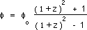
pero con :

(16)

y el tamaño angular obedece a :

(17)

Cuando z tiende al infinito, f tiende a una constante, un comportamiento claramente diferente y en acuerdo cualitativo con los datos.

(18)

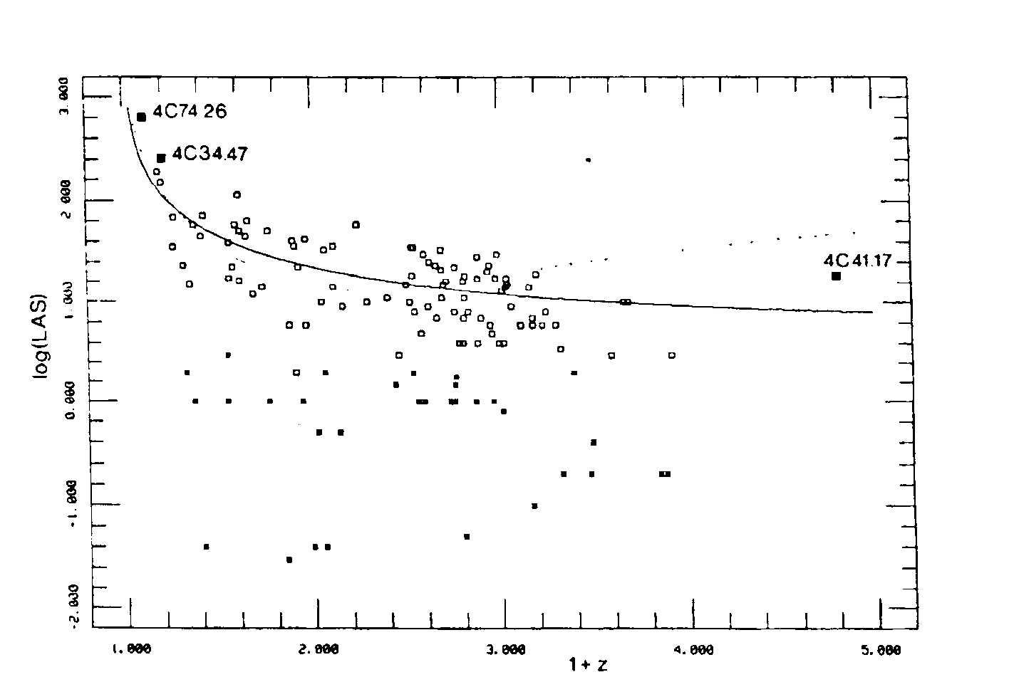
Fig 18: El mayor tamaño angular (LAS, en segundos de arco), en una escala logarítmica en función del corrimiento al rojo para las 95 fuentes extendidas con morfologías "T", "D1" y "D2" (cuadrados) y las 33 fuentes compactas con morfologías "SSC" (asteriscos). Las dos curvas representan los ajustes del modelo de gauge (línea continua) y del modelo de Einstein-de-Sitter (línea punteada) obtenidos para las fuentes extendidas en este artículo. Tres otras fuentes radio de gran extensión se muestran como comparación. 4C41.17 siendo la galaxia más lejana conocida actualmente, 4C74.26 la mayor fuente radio asociada a un quásar.

...Para comparar cuantitativamente la calidad del ajuste de los dos modelos a los datos, escribamos f = f₀f(z) donde f(z) es una función característica predicha anteriormente por cada modelo. Se realizaron regresiones lineales entre f(z) y los datos de "mayor tamaño angular" [LAS después de BM], ya sea para la muestra completa de 134 QSO, ya para una muestra reducida de 83 QSO en la cual solo se seleccionaron los objetos con lóbulos bilaterales, es decir, aquellos con morfologías "T" o "D1" definidas por BM, excluyendo así los núcleos con espectro abrupto o "SSC" y las fuentes con lóbulos unilaterales o "D2", con el fin de probar posiblemente propiedades diferentes entre fuentes compactas y extendidas. Los resultados de las regresiones son los siguientes, todos los coeficientes lineales dados y sus barras de error RMS expresados en segundos de arco:

• con el modelo de Einstein-de-Sitter :

F = (28,8 ± 2,9) f(z) - (89,3 ± 20,1)

para la muestra completa, y

F = (31,3 ± 3,3) f(z) - (90,5 ± 20,8)

para la muestra reducida.

• con el modelo de gauge :

F = (21,5 ± 2,11) f(z) - (19,1 ± 19,6)

para la muestra completa, y :

F = (24,3 ± 2,3) f(z) - (17,3 ± 19,8)

para la muestra reducida.

...Es claro que el nuevo modelo de gauge proporciona un ajuste claramente mejor a los datos, ya que cualquiera que sea la muestra, el término constante moderado que implica es marginalmente significativo desde el punto de vista estadístico, y por lo tanto el valor (esperado) cero es muy probable. La situación es completamente opuesta con el modelo clásico, ya sea cual sea la muestra, ya que el término constante es fuertemente significativo desde el punto de vista estadístico y su valor grande y negativo es inaceptable desde el punto de vista teórico, a menos que se suponga que efectos sistemáticos muy fuertes, como los sospechados anteriormente, estén en juego en los datos.

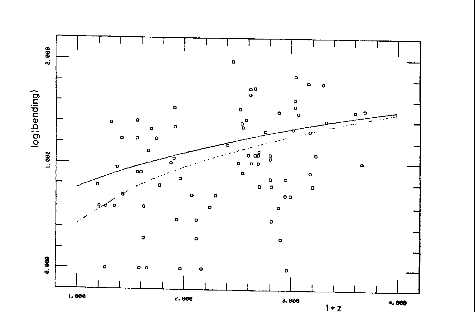
3b. La curvatura.

...Mostremos también que la apariencia más curvada, más deformada de los QSOs lejos señalada por BM puede ser curiosamente explicada por el nuevo modelo de gauge, siempre que no se trate de un artefacto resultante de diversos efectos sistemáticos. Puesto que en el nuevo modelo se supone que todas las energías se conservan durante el proceso de gauge cósmico, podemos incluir la conservación de la energía de rotación del núcleo del QSO emitiendo los chorros: (19)

Como m » R, I » R³ y W » R⁻³/² W » 1/t » (1 + z)³/², en curiosa concordancia con el ajuste a ley unidimensional inferior efectuado por BM sobre la muestra reducida (ya que la curvatura solo se define en este último caso), es decir:

(20)

Fig 21: La curvatura (en grados) en una escala logarítmica en función del corrimiento al rojo para las 83 fuentes extendidas con morfologías "T" y "D1" solamente, para las cuales está definida. La curva continua corresponde al ajuste del modelo de gauge, indicando que las velocidades angulares eran más altas en el pasado, mientras que la línea punteada representa el ajuste en ley potencia de Barthel y Miley (BM).

...Ahora, propongamos una explicación somera, refiriéndonos al análisis reciente de Greyber [5] sobre la naturaleza de los motores centrales en los QSOs responsables de sus tasas de producción de energía enormes: si aceptamos el hecho (i) de que los paquetes de plasma son eyectados a gran velocidad del motor central, de forma continua o no, a lo largo del eje del dipolo magnético de los QSOs, y (ii) que este último no es generalmente coincidente con el eje de momento cinético, entonces nos enfrentamos a un modelo similar a un aspersor rotativo, en el cual los chorros se curvarán en una especie de espiral de Arquímedes, siempre que la interacción con el MIG permanezca despreciable. Y aunque esta interacción se vuelva significativa a cierta distancia del núcleo, los chorros dejarán de expandirse allí, causando un aumento en la curvatura. Puesto que no hay razón para que la densidad del MIG esté distribuida esféricamente alrededor de los QSOs, tales interacciones podrían explicar las asimetrías frecuentes observadas en sus chorros, así como efectos aleatorios en la curvatura global, como se discutió por BM.

...Como consecuencia, cuanto mayor sea el corrimiento al rojo del QSO, mayor será su velocidad angular debido al proceso de gauge cósmico, y por lo tanto mayor será la curvatura de sus chorros.

4. CONCLUSIÓN.

...Nos hemos concentrado en características específicas recientemente destacadas en la distribución de los tamaños angulares y la curvatura en función del corrimiento al rojo para un conjunto homogéneo de 134 QSOs radio. Encontramos interesantemente que nuestro modelo de gauge con "constantes variables" proporciona un mejor ajuste a estas distribuciones que el modelo clásico de Einstein-de-Sitter, siempre que (i) las tendencias observadas (tamaños angulares más pequeños y curvaturas más grandes para los QSOs lejos) sean confirmadas por observaciones futuras, (ii) que estas tendencias no estén dominadas por diversos efectos o artefactos, y (iii) que las suposiciones simples hechas sobre ciertos mecanismos involucrados sean reales. Además, se necesitan investigaciones adicionales sobre la potencia intrínseca de estas fuentes para comprender si el modelo de gauge permite una mejor comprensión de las tendencias observadas, es decir, que la luminosidad de los QSOs lejos sea mucho mayor que la de los QSOs cercanos.

5. REFERENCIAS.

[1] J.P. PETIT : Interpretación del modelo cosmológico con velocidad de la luz variable. Modern Physics Letters A, Vol. 3, n° 16, noviembre 1988

[2] J.P. PETIT : Modelo cosmológico con velocidad de la luz variable. La interpretación de los corrimientos al rojo. Modern Physics Letters A, Vol. 3, n° 18, diciembre 1988.

[3] P.D. BARTHEL & G. K. MILEY. Evolución de la estructura radio en los cuásares: una nueva sonda de las proto-galaxias? - Nature Vol 333, 26 mayo 1988.

[4] M.L. NORMAN, J.O. BURNS y M.E. SULKANEN : Perturbación de los chorros radio galácticos por los choques en el medio ambiente, Nature 335 (1988) 146.

[5] H.D. GREYBER : La importancia de los campos magnéticos intensos en el Universo, Comments Astrophys. 13 (1989) 201.